Posts under category statistics homework help

The Open University Statistics - M248 TMA 03

Please read the Student guidance for preparing and submitting TMAs on the M248 website before beginning work on a TMA. You can submit a TMA either by post or electronically using the University’s online TMA/EMA
service.

You are advised to look at the general advice on answering TMAs provided on the M248 website.
Each TMA is marked out of 50. The marks allocated to each part of each question are indicated in brackets in the margin. Your overall score for each TMA will be the sum of your marks for these questions.

Note that the Minitab files that you require for TMA 03 are not part of the M248 data files and must be downloaded from the ‘Assessment’ area of the M248 website.

Question 1, which covers topics in Unit 5, and Question 2, which covers topics in Unit 6, form M248 TMA 03. Question 1 is marked out of 28; Question 2 is marked out of 22.

You should be able to answer this question after working through Unit 5.
(a) In this part of the question, you should calculate the required probabilities without using Minitab, and show your working. (You may use Minitab to check your answers, if you wish.)

In England, the most serious emergency calls requesting an ambulance are classified as ‘Red 1’. According to data from NHS England, in March 2017, the London Ambulance Service (LAS) received a total of 1597 Red 1 emergency calls. Based on this number and adjusting for variations during the day, suppose that Red 1 calls arriving at LAS in daylight hours may be modelled as a Poisson process with rate 3 per hour.

(i) (1) Write down the distribution of the number of Red 1 calls arriving at the LAS in a 30-minute period during daylight hours, including the values of any parameters. [2]

(2) Calculate and report the probability that three Red 1 calls arrive at the LAS in 30 minutes during daylight hours. [2]

(ii) (1) Write down the distribution of the waiting time (in hours) between the arrival of two successive Red 1 calls at the LAS during daylight hours, including the values of any parameters. [2]

(2) Calculate and report the probability that the gap between the arrival of two successive Red 1 calls at the LAS during daylight hours will exceed 20 minutes. [4]

(b) This part of the question concerns data on the lengths of the 51 time intervals (in days) between successive earthquakes in California starting from a major earthquake on 9 January 1857, up to an earthquake on 24 August 2014. (To qualify for inclusion in this dataset, earthquakes had to be single mainshocks with magnitude of at least 4.9.) These time intervals are in the variable Interval in the worksheet california-earthquakes.mtw. In this part of the question, you will explore whether or not a Poisson process is a suitable model for these data.

(i) The intervals between successive events in a Poisson process are exponentially distributed. Using Minitab, find the mean and standard deviation of the intervals between earthquakes in California. Are these values consistent with the data being observations from an exponential distribution? Give a reason for your answer. [3]

(ii) Using Minitab, obtain a histogram with the following properties:
• the ticks on the horizontal axis are at the cutpoints
• the bins have width 500 days
• the first bin starts at 0 days and the last bin finishes at 7500 days. Include a copy of your histogram in your answer. Is the shape of the histogram consistent with the data being observations from an
exponential distribution? Give a reason for your answer. [4]

(iii) The data are listed in the order in which they arose. Using Minitab, produce an appropriate graph to investigate whether, for the period of observation, the data are consistent with the rate at which earthquakes occur in California remaining constant. Include a copy of your graph in your answer. On the basis of your graph, explain whether or not you think that the rate at which earthquakes occur in California remained constant over the course of the period studied. If you think that the rate did not remain constant, then say how you think it changed. [6]

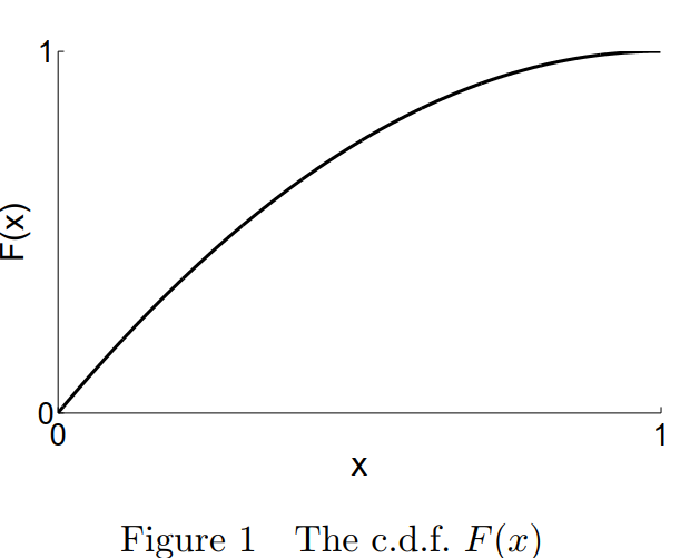
(c) A certain form of ‘triangular’ distribution has c.d.f.
F(x) = 1 − (1 − x)2; 0 < x < 1;
which is plotted in Figure 1 below. (It is called a triangular distribution because its p.d.f. is a line which, together with the axes, forms a triangle.)
2023-04-04T09:09:09.png

(i) Calculate the value of the upper quartile for this distribution. [3]
(ii) On a copy of, or very rough sketch based on, Figure 1, show the values of α and its corresponding quantile qα for the upper quartile that you calculated in part (c)(i). [2]

Question 2
You should be able to answer this question after working through Unit 6.
(a) In this part of the question, you should calculate the required probabilities using tables, and not Minitab, and show your working.

(You may use Minitab to check your answers, if you wish.)
A model for normal human body temperature, X, when measured orally in ◦F, is that it is normally distributed, X ∼ N(98:2; 0:5184).
(i) According to the model, what proportion of people have a normal body temperature of 99 ◦F or more? [3]
(ii) Find the normal body temperature such that, according to the model, only 10% of people have a lower normal body temperature. [2]
(iii) Let W denote normal human body temperature, when measured orally in ◦C. Given that W = 5 9(X − 32) and that
X ∼ N(98:2; 0:5184), what is the distribution of W ? [3]
(iv) According to the model you just derived for W , what proportion of people have a normal body temperature of between 36 ◦C and 36.8 ◦C? [4]

(b) The Minitab file body-temperature.mtw contains values of the normal body temperature, measured orally, of n = 130 people. The model for normal human body temperature used in part (a) of this
question was obtained partly by consideration of these data. The data can be used to check whether or not the assumption of normality of normal human body temperature is appropriate. Suggest a suitable graph to investigate specifically whether or not a normal distribution might be a good model for the normal body
temperature of people, measured orally. Using Minitab, produce this graph. Include a copy of your graph in your answer. On the basis of this graph, do you think that a normal distribution is a plausible model for
these data? Explain your answer. [5]

(c) Suppose that the mean weight of a particular type of ripe tomato is 155 g and the variance of the weight of this type of ripe tomato is 576 g2. A random sample of n = 36 such ripe tomatoes is obtained.
(i) What is the approximate distribution of the sample mean weight of the random sample of 36 ripe tomatoes? [2]

(ii) Use Minitab to find the probability that the sample mean weight of the sample of 36 ripe tomatoes lies between 150 g and 157.5 g. To show that you used Minitab, write down the results of any intermediate calculations you make in Minitab to the same number of decimal places as given by Minitab. [3]

Our statistics help experts have prepared the following sample solutions for you to compare.

M248 TM 03 open university statistics solutions for question 2.docx

The Open University Statistics TMA02

Question 1 - 27 marks
You should be able to answer this question after working through Unit 3.
(a) In 1986, the US Space Shuttle Challenger tragically exploded in flight. This accident was caused by the catastrophic failure of rubber ‘O-ring’ seals that linked segments of its rocket boosters together. There were six O-ring seals in Challenger (and all other Space Shuttles at the time). Table 1 shows the numbers of O-ring seal failures that had occurred on each of 23 previous Space Shuttle flights.

Table 1 Number of O-ring seal failures
2023-04-04T08:27:45.png

(i) Let p be the probability that an O-ring seal fails on a flight. What distribution is appropriate to describe the failure or non-failure of a particular O-ring seal on a particular flight? (Ensure that you
define the corresponding random variable appropriately.)

(ii) A reasonable estimate of p is 3=46 ’ 0:065. Explain where this number comes from.

(iii) It is suggested that an appropriate model for the number of O-ringseals that fail on a particular flight might be a binomial distribution B(6; p). What assumptions are made by using thismodel? In your opinion, is a binomial model appropriate? Briefly justify your answer.

iv) Use Minitab to obtain a table containing both the p.m.f. and c.d.f. of the B(6; p) distribution with p = 0:065. (Do not change the number of decimal places of the values obtained from those provided by Minitab.)

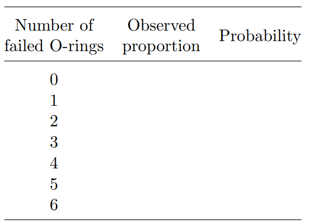
(v) Use the information in Table 1 and the solution to part (a)(iv) to complete the following table, giving your values rounded to three decimal places.

2023-04-04T08:31:39.png

Comment briefly on how close the observed proportions of flights on which 0; 1; 2; : : : ; 6 O-ring seals failed are to those predicted by the binomial model. What does this suggest about the appropriateness, or otherwise, of the binomial model?

(b) Records show that 6% of blood samples tested for a certain condition test positive. Assuming that whether or not a blood sample tests positive is independent of whether or not any other blood sample tests
positive, calculate by hand the following probabilities correct to four decimal places. In each case, state clearly the probability model that you use (including the values of any parameters) and show your working.

(i) The probability that, out of 20 samples tested, at least three will test positive. [6]
(ii) The probability that the first blood sample that tests positive tomorrow will be the ninth sample tested. [3]

(c) The number of flaws in a fibre optic cable follows a Poisson distribution with parameter λ = 1:25. Calculate by hand the probability that there are two or fewer flaws in such a fibre optic cable, giving your answer correct to three decimal places. Show your working.

Question Two
You should be able to answer this question after working through Unit 4.
(a) In Question 2(b) of TMA 01, the probability mass function of a discrete random variable X representing the number of bicycles available at a docking station each morning was introduced. This p.m.f. is repeated
here, in Table 2.

2023-04-04T08:34:35.png

(i) What is the mean number of bicycles available at the docking station each morning? [2]
(ii) What is the variance of the number of bicycles available at the docking station each morning?

(b) The Atacama Desert in Chile is known as the driest place on Earth. Suppose that in one part of the Atacama Desert, whether it rains at all in a given year has probability 0.2 and that whether or not it rains in one year is independent of whether or not it rains in any other year.

Answer the following questions, in each case stating clearly the probability model that you use (including the values of any parameters).

(i) Suppose that a random variable X is defined to take the value 1 when there is rainfall in a particular year and 0 when there is not.
What is the mean of the random variable X? [2]
(ii) What is the expected number of years with some rainfall in a period of 100 years? [2]
(iii) What is the expected value of the number of years up to and including the first year in which there is some rainfall? [2

(c) A scout on a camping trip is requested to find some dry sticks of length
at most one metre to use as firewood. A model for the distribution of
the lengths, X, in metres, of sticks that she brings back to the camp has
probability density function
f(x) = 3
2
px; 0 < x < 1:
(i) According to the model, what is the mean length of the sticks that the scout brings back? [3]
(ii) According to the model, what is the standard deviation of the lengths of the sticks that the scout brings back? [5]
(iii) What are the units of the mean and the standard deviation that you have just calculated? [1]

(d) The number of customers buying a cooked breakfast at a high-street cafe on a weekday morning is a random variable X with mean 24 and variance 36. As a loss leader { a product sold at a loss to attract
customers to also partake of its other offerings { the cafe charges $3:50 per breakfast and has fixed breakfast-specific daily costs (ingredients, labour) of $105. Let Y be the cafe’s daily loss on breakfasts, in pounds, where Y = 105 − 3:5X: What are the mean and standard deviation of this loss? [3]

Solution for the first question has been attached here for your reference, TMO2 Open university statistics.docx
Let us no if you need further help with your statistics.

Complete the following paragraph by selecting words

You should be able to answer this question after working through Unit 2.
(a) Complete the following paragraph by selecting words or phrases from the list that follows it to fill in the underlined gaps.

In a long sequence of repetitions of a study or experiment, random samples tend to settle down towards probability distributions in the sense that, for discrete data, bar charts settle down towards probability functions and, for continuous data, histograms settle down towards probability functions. As the sample size increases, the amount of difference between successive graphical displays obtained from the data .

Available words and phrases: continuous cumulative decreases density discrete
frequency increases mass model models relative frequency remains constant unimodal unit-area [3]

(b) Kevin lives in a city which operates a bicycle hire scheme using a large number of bicycle ‘docking stations’ spread around the city. He walks past a small docking station, for up to six bicycles, each morning. Kevin has come up with the following probability mass function (p.m.f.) for the distribution of the random variable X which denotes the number of bicycles available at the docking station each morning.
It is given in
Table 1.
Table 1 The p.m.f. of X

x 0 1 2 3 4 5 6
p(x) 0.3 0.2 0.2 0.1 0.1 0.05 0.05
(i) What is the range of X? [1]
(ii) Explain why the p.m.f. suggested by Kevin is a valid p.m.f. [2]
(iii) What is the probability that, on any particular morning, there is one bicycle at the docking station? [1]
(iv) Write down a table containing values of F(x), the cumulative distribution function (c.d.f.) of X, for x = 0; 1; 2; 3; 4; 5; 6. [2]
(v) Write the probabilities P(X < 3) and P(X ≥ 5) in terms of the c.d.f. F(x). Use the c.d.f. to calculate the values of these two probabilities.

(c) In 1955, C.W. Topp and F.C. Leone introduced a number of
distributions in the context of the statistical modelling of the reliability of electronic components in engineering. One of these distributions has probability density function (p.d.f.) given by f(x) = 4x(1 − x)(2 − x) on the range 0 < x < 1.
(i) Verify, by integration, that Integrate( 4x(1 − x)(2 − x)) dx = x2(2 − x)2 + c; where c is an arbitrary constant

(ii) Explain why the p.d.f. suggested by Topp and Leone is a valid
p.d.f. [4]
(iii) What is the c.d.f. associated with this p.d.f.? [2] (iv) Suppose that X is a random variable following this p.d.f., and that we are interested in evaluating P(1/3 < X < 2/3). Write this probability in terms of the c.d.f., and hence show that P (1/3 < X < 2/3)= 39 81
(which is approximately 0.481)

The Open University Statistics TMA 01 Question 1
(a) A number of Japanese black pine tree seedlings were planted in a rather inaccessible location to which researchers returned at the same time each year in order to measure their growth. The resulting data comprise the height of the young trees (measured on an effectively continuous scale of millimetres) and the age of the trees (1, 2, 3 or 4 years).

(i) Name two graphical displays which are suitable for studying the distribution of the heights of the trees at age 1 year. Give a single reason for the suitability of both displays. [3]

(ii) Unfortunately, the young trees were susceptible to dying off, so the number of trees that remain alive at each age is also a variable of interest. Name a graphical display which is suitable for showing the number of trees alive at each age. Give a reason for your answer. [2]

(iii) Name two graphical displays which are suitable for studying the way that the heights of the trees depend on their ages. Give a separate reason for the suitability of each display. [4]

(b) The Minitab worksheet snow-depth.mtw contains measurements of the depth of snow lying at each of n = 114 locations on an Antarctic ice floe in March 2003. The measurements are in centimetres, rounded to
the nearest whole number. The data are in the variable Depth.

(i) Produce Minitab’s default frequency histogram for Depth. Include a copy of this histogram in your answer. Briefly describe the main features of the distribution suggested by this histogram. [3]

(ii) Now use Minitab to produce a frequency histogram for Depth with cutpoints at 0, 10, 20, . . . , 100 cm. Include a copy of this histogram in your answer. Briefly describe the main feature of the
distribution according to this histogram and state why this histogram gives a more clear-cut picture than the default histogram that you obtained in part (b)(i). [4]

(iii) Now use Minitab to produce a unit-area histogram for Depth with cutpoints at 0, 10, 20, . . . , 100 cm. Include a copy of this histogram in your answer. In what way(s) does this histogram differ from the frequency histogram that you obtained in part (b)(ii)? The heights of the bars in the histogram that you have just produced should be 0:005 0:016 0:018 0:012 0:011 0:019 0:012 0:004 0:002 0 (each given correct to three decimal places except the last which is exact). Use this information to verify that this histogram does have unit area, as claimed. [5]

(iv) Using Minitab, obtain the sample size, sample mean and sample median of the variable Depth and report your result, by copying Minitab text, in the form

Variable N Mean Median
Depth . .*
(where, of course, the asterisks are replaced by numbers).
Comment briefly on the relative size of the sample mean and the
sample median, relating your comments to the shape of the
histogram that you obtained in either part (b)(ii) or (b)(iii). [4]
This question was solved by our experts under our pay someone to do my statistics homework statistics help services. Note that this question requires you to use Minitab to solve the assignment by hand while using Minitab where necessary. we have attached solutions for the first question here for you reference. TM01 Open University Statistics solutions.docx. You can contact us if you need further help with your coursework assignments.

This question is intended to assess your understanding of point estimation.
You should be able to answer this question after working through Unit D1.
(a) The data in Table 4 relate to the classification of 134 recorded crimes(occurring during a month in a certain UK postcode area) into five crime categories.

Table 4    Classification of crimes
 Crime categories    1    2    3    4    5
Observed frequency    25    14    42    11    42

A possible model for these data is the one indexed by a parameter θ, where 0 < θ < 1, with the following probabilities of categories 1,2,3,4,5, respectively:
2023-04-04T07:55:45.png

(i) Show that the likelihood of θ for these data has the form
2023-04-04T07:56:19.png,
where c is a number and does not involve θ. (You should show how
c is formed, but you do not need to evaluate its value.)
(ii) Ignoring c, the log-likelihood is [4]
2023-04-04T07:56:52.png.
Use MINITAB to evaluate l(θ) at θ = 0.05,0.10,0.15,... ,0.95.
Give the values of l(θ) in a table, and produce a graph in which
l(θ) is plotted against θ for each of these values.
(iii) Correct to two decimal places, the value of θ that maximizes l(θ) is 0.90. Find θb, the maximum likelihood estimate of θ, correct to three decimal places. Include sufficient detail in your answer to [6]