Posts under category statistics homework help

Analysis of a Fitted Multiple Regression Model

If your “best model” selected in the previous chapter contains more than one x-variable, run that regression model in SAS. If it only has one x-variable, use the best model that had more than one x-variable. Answer the following questions.

  1. Analysis of Output
    (a) The t-tests
    (i) What is being tested?
    (ii) What are the results of the tests? (Careful, these are partial coefficients.)

(b) The F-test

(i) State the null and alternate hypotheses for your model. 
(ii) State the conclusion of the test and the grounds for the decision.

(c) The -equation

    (i) State the equation for your fitted model;
 (ii) Explain how is related to the E(YX).
  1. R-square
    (a) Report the value of R-square;
    (b) Show how it was computed from the software output;
    (c) Explain the meaning of your R-square using the approach found in Lecture Notes 5.
    (d) Give the naïve interpretation of your R-square, as discussed on LN5.
  2. Adjusted R-square
    (a) Report the value of the adjusted R-square;
    (b) Show how it was computed from the output;
    (b) What is the meaning of your adjusted R-square value?
  3. The Partial Regression Coefficients
    (a) Run the simple regression of y on one of your x-variables from your best model to show that this produces a sample slope coefficient that differs from the partial sample slope coefficient for the same x-variable when your other x-variables are in the model.
    (b) Describe the steps by which you can use a series of regressions to compute the above partial regression coefficient for the selected x-variable, above. This involves regressing y on those other x-variables, saving the residuals, and so on, until finally you regress one set of residuals on a second set of residuals.
    (c) Demonstrate that what you described in (b) actually works!
    (d) Output from SAS the partial R-square and the partial correlations coefficient for the same x-variable on which you analyzed the partial coefficient in your best model.
    (e) Using the same approach as in (c), show that the ordinary R-square for the regression of those residuals yields the partial R-square. Likewise for the partial correlation coefficient.
  4. Model Diagnostics
    (a) Explain what is shown by Cook’s distance diagnostic plot for your model.

Chapter 7
Run a ridge regression analysis of your data. Try in your own words to explain what that technique does and interpret the output. Supply your own Headers.
Build a regression model to explain the price of the house
Save the file as: MKT9740_LastName when you submit. I would prefer if you submit the file as PDF.
Answer the questions as clearly as possible with the main results and findings explained as your response. You can append the SAS code and other analysis as an Appendix.
Do not email me SAS files or SAS Codes separately. Copy and paste the output nicely and refer to the output as you see fit as an Appendix.
Use “Equation” option in Word to write models, if necessary.

Question 1

Download the data set on 401K contribution of individuals (401subs.xls). The description of the different variables is given below:

Variable Description
e401k This equal 1 if the individual is eligble for 401(k) contribution.
inc The income level of the individuals in thousands of $ ($1000).
married This equal 1 if the individual is married.
male This equal 1 if the individual is male
age Age of the individual.
fsize The family size of the individual
netfina The net financial assets of the individual in thousands of $ ($1000).
p401k This equal 1 if the individual participates in the 401(k) program.
pira This equal 1 if the individual participates in an IRA program.
incsq Square of the income.
agesq Square of the age.

  1. Build a regression model to explain the net financial assets of an individual. The explanatory/independent variables you can use are age, income, family size, whether the individual is married, male, participates in 401k etc. Summarize your findings providing detailed explanations. What do you find that is interesting.
  2. Can you include both p401k and pira as explanatory variables at the same time in a model to explain the net financial assets of an individual? Why or why not? Explain clearly using analysis as needed.
  3. Based on your model, what is the expected net financial assets of an individual who is 45, has a family size of 4, is married, is male and has an income of $50 (in thousands)? You can use the mean of the other additional variables if you are using them in your model. You may make any other reasonable assumptions.

Question 2
Download the data set on house prices (Hprice.xls). The description of the different variables is given below:

Variable Description
price House price, in thousands of $($1000s)
assess Assessed value, in thousands of $($1000s)
bdrms Number of bedrooms in the house
lotsize Size of lot in square feet
sqrft Size of house in square feet
colonial This equals 1 if home is colonial style
lprice Log(price)
lassess Log(assess
llotsize Log(lotsize)
lsqrft Log(sqrft)

  1. Build a regression model to explain the price of the house. The explanatory variables that need to be used are the number of bedrooms, lot size, home size and whether the house is a colonial. Summarize your findings. Does this model make sense?
  2. Perform the various regression diagnostics to make sure that the model is appropriate. Report your findings.
  3. Now redo/re-estimate the model by using log(price), log (assess), log(lotsize) and log (sqrft) in place of price, assess, lot size and sqrft. Also perform the various regression diagnostics. Summarize your findings.
  4. Do the assessed values accurately reflect the actual value of the price?

Question 3
Download the data set-apples (apples.xlxs). This data set contains individuals’ purchase of regular and eco-labelled (e.g., organic) apples along with other relevant variables. The description of the different variables is given below:

Variable Description
id Identifier of the individual
educ Education level in terms of the number of years of schooling
date date: month/day/year
state home state
regprc price of regular apples $/lb
ecoprc price of eco-labeled apples $/lb
inseason =1 if the individual was surveyed about apples in November
hhsize household size of the individual
male =1 if individual is male
faminc family income, thousands of $
age Age of the individual
reglbs quantity of regular apples purchased by the individual in pounds
ecolbs quantity of regular apples purchased by the individual in pounds
numlt5 Number of people in the individual’s household younger than 5 years old
num5_17 Number of people in the individual’s household with ages from 5-17
num18_64 Number of people in the individual’s household with ages from 5-17
numgt64 Number of people in the individual’s household with ages from 5-17

  1. From the above, choose the variables that you think are relevant for modeling the sales of regular and eco-labelled apples (i.e., reglbs, ecolbs). Present the summary statistics of the relevant variables (and also the sales of regular and eco-labelled apples).
  2. Estimate the regression model to explain the sales of regular apples. That is, run the regression model with sales of regular apples as the response/dependent variable and the variables you have chosen (in #1 above) as the dependent/explanatory variables.
  3. Calculate the (own price) elasticity of regular apples. Do this for the Linear model, Semi-Log model and the Log-Log model.
  4. Calculate the (own price) elasticity of eco-labelled apples. Do this for the Linear model, Semi-Log model and the Log-Log model.
  5. Calculate the cross-price elasticity of regular apples and the cross-price elasticity of eco-labelled apples. You can do this for just one model.

            Homework Assignment #3
            First assignment on Semester Project
             

As the first step in your Regression Project, find a data set that is of interest to you. The data set should contain at least 50 rows of data and have a y-variable and an x-variable for now, and at least 4 x-variables as regressors later on (to make the "model selection" sections interesting). Some possible sources of data sets are given in the posted guide.
However, if you do not readily find a data set, do not waste all weekend trying to find the "perfect" data set. Rather, just grab some baseball data (but not mine) or some quarterly Bureau of Labor Statistics data and use that for this assignment. Then, if you decide to use something different for your project, you will find it is fairly easy to redo this assignment for inclusion in your project, because you will have already have done the assignment once.

For the SAS and R questions, you are free to insert your data (and change the variable names) of the SAS and R templates given in the lecture notes.

Imbed all graphs and tables in the document. Do NOT put them on separate pages, as the reader will soon give up looking for them.

This homework, and all the following homework, will be drafts of chapters of your semester project. Therefore, with that goal in mind, please structure as follows:
(1) show the given chapter headings, such as
Chapter 1
(b) show the given underlined section headers, such as

  1. Scatterplots,
    (c) do NOT show the questions asked: just answer them! That means, that the answer has to include the question. Example: “Why are you going home?” A good answer: “I am going home to feed the dog.” A weak answer: “To feed the dog.”

Show Title: A Multiple Regression Analysis of

Show your Name: _

Chapter 1

 1. Topic

The subject of this study is to investigate the relationship between sale price of houses and its lost size. The purpose is to inform my future house purchasing decision, to effectively predict the probable cost of a house given its characteristics. The goal is to effectively purchase a house having determined the range within which its true price is likely to fall.

  1. Data Source
    The dataset is obtained from Rdata sets directory available at Github.io.

https://vincentarelbundock.github.io/Rdatasets/datasets.html
https://raw.githubusercontent.com/vincentarelbundock/Rdatasets/master/csv/Ecdat/Housing.csv

  1. Variables

The data set has 546 observations (n = 546) and 13 variables. The variables in this dataset are:
Price (sale price of a house)

Lotsize (the lot size of a property in square feet)

Bedrooms (number of bedrooms)

Bathrms (number of full bathrooms)

Stories (number of stories excluding basement)

Driveway (does the house has a driveway ?)

Recroom (does the house has a recreational room ?)

Fullbase (does the house has a full finished basement ?)

Gashw (does the house uses gas for hot water heating ?)

Airco (does the house has central air conditioning ?)

Garagepl (number of garage places)

Prefarea (is the house located in the preferred neighbourhood of the city ?)

  1. Data View

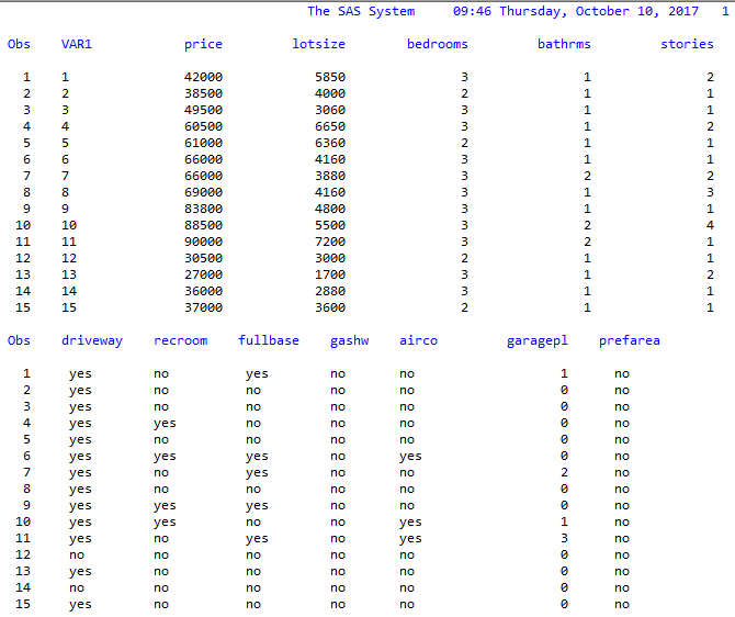
sas data view.png

The first 15 observations are displayed above.

Chapter 2 A Simple Regression Model

  
  Predicting house price using its lot size. x=lot size, y=price.
SAS output
  1. Scatterplots

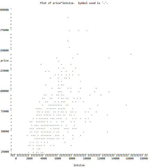
sas scatterplots.png

Scatterplot of price vs. lot size.

  1. Analysis of Scatterplot
  2. The Linear Regression Model
    State your regression model and briefly explain

The regression model is:
(a) the meaning of your YX term in the model;
(b) how the terms on the right-side are related to E(YX);
(c) how the terms on the right-side are related to V(YX).

  1. SAS Output for the Fitted Model

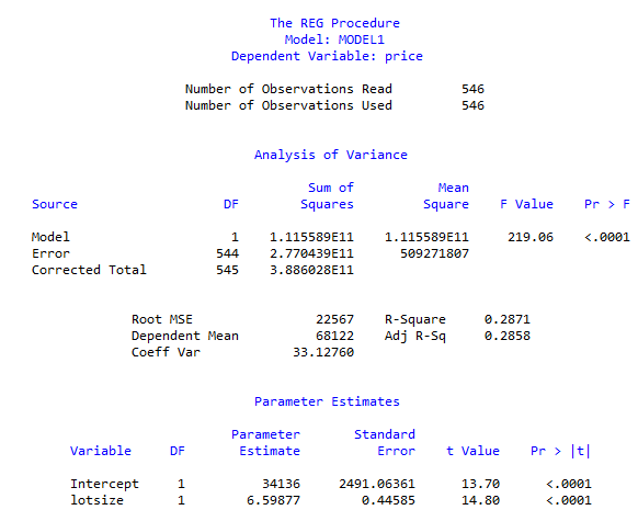
the proc reg SAS model.png
Run Proc Reg in SAS to fit your model. Show the table output, cleaned-up, and the SAS regression plot with the confidence and prediction bands. Otherwise, only show what you are going to use.

  1. Analysis of Output
    (a) The t-tests
    (i) What is being tested?
    (ii) What are the results of the test?
    (iii) Use the Story of Many Possible Sample to explain how the test is done.

(b) The -equation

    (i) State the equation for your fitted model;
 (ii) Explain howis related to E(YX) using the story of many possible samples.

(c) In the regression plot, explain what is being shown by the 95% confidence band and the 95% prediction band. Include a vertical x-cut to provide a focus for your explanation.

A)
Download the excel dataset name online_buying. The dataset consists of purchases made by consumers across two channels from a company/firm: online and the physical store (multi-channelpurchases). More specifically, the dataset has following columns:

1) Customer: The Id of the customer.
2) Online_buy: This takes the value of 1 if the consumer buys online and 0 if he/she buys in
the physical store.
3) distance: The distance in miles from the customers home/residence to the physical store.
4) experience: The number of months that the customer has been shopping with the firm.
Thus, this can be interpreted as the experience the customer has with the firm.

5) c_rank: This is the convenience rank. Customers were asked about how convenient it
would be for them to shop online versus the physical store on a scale from 1(least
convenient) to 4 (most convenient).

  1. Formulate and estimate a (logistic) model to understand how the factors can affect the likelihood of customers shopping online. Comment on the model parameter estimates. You can calculate the odd ratios etc. What are the managerial implications of your findings?
  2. For each customer calculate the probability of him/her shopping online. You should do this based on the model estimates and the data and using the formula for p. You can do this either in excel or in SAS.

B)
Download the excel dataset brand_choice**. You have disaggregate data of choice of brands (denoted by 1, 2 and 3) in the beverage category by 50 consumers. Let’s say brands 1, 2 and 3 are Fuze, Honestea and Suja respectively. The data set consists of the following:

1) Customer_id: This denotes/indexes the customer who is making the purchase.
2) Price: This indicates the price per 12 oz. of the brand.
3) Brand: If the particular brand is chosen by the customer, then this takes the value of 1; if the brand is not chosen then this takes the value of 0.
4) Product: This number tells you which brand it is: brands 1, 2 and 3 are Fuze, Honestea
and Suja respectively.

The objective is to model the consumer’s choice of beverage brands using
brands’ pricing information. Estimate the model and interpret the results of the model.
Note: You should use proc mdc to do this.
You can modify the code given below and use it. You should first generate the intercept terms in the data for each of the products.

You can do this as follows.
In cases when product=1 then you can have int1=1 and when product=2 and product=3 then int1=0
· When product=2 then you can have int2=1 and when product=1 and product=3 then
int2=0
· When product=3 then you can have int3=1 and when product=1 and product=2 then
int3=0
So int1=1 for product 1 only and 0 otherwise; int2=1 for product 2 only and 0 otherwise; int3=1 for product 3 only and 0 otherwise. You can do the above in excel or SAS.

           proc sort data=brand_choice;
           by customer_id;
           run;
           proc mdc data=brand_choice;
           model brand = in1 in2 price /
           type=clogit
           nchoice=3;
           id customer_id;
           run;

C)

Please read the article attached (“Retailers’ Emails Are Misfires for Many Holiday Shoppers”)
and answer the following questions.

1) In your own words, what does it mean to 'personalize' digital messaging? What tools,
technologies and methods are necessary to personalize digital messaging?

2) The article says “the ugly truth is that most retailers haven’t done the unsexy work of
understanding how to use the data”. How can retailers use the data available to them to
better design personalized emails? What should they do? How can customers be targeted with the right product?

https://www.wsj.com/articles/retailers-emails-are-misfires-for-many-holiday-shoppers-1511778600

Understanding Mixed Effects Models

Qn1. A mixed model is “mixed” because it contains both between-subjects and within-subjects factors.

True
False

Qn2. Which of the following best describes fixed effects?

Fixed effects are manipulated factors whose levels are sampled randomly from a larger population of interest
Fixed effects are random factors whose chosen levels are of explicit interest.
Fixed effects are random factors whose levels are sampled randomly from a larger population of interest    
None of the above

Qn3. Random effects are called “random” in part because their levels are randomly sampled form a larger population about which wish to generalize

True
False

Qn4. Linear mixed models (LMMS) can handle Poisson response distributions.

True 

False
Qn5. Which is not an advantage of a linear mixed model (LMM)

The ability to handle within-subjects factors
The ability to handle unbalanced designs
The ability to handle missing data
The ability to handle non-normal response distributions
The ability to handle violations of sphericity

Qn6. Linear mixed models (LMMs) produce small residual degrees of freedom.

True
False

Qn7. Nesting is useful when the levels of a factor are not meaningful when pooled across all levels of the other factors.

True
False

Qn8. Nesting is necessary when we wish to calculate the means and variances of a nested factor’s levels only within the levels of the other factors, that is, the nesting factors.

True
False

Qn9, Linear mixed models (LMMs) generalize the linear model (LM) to non-normal response

True 
False

Qn10. Generalized linear mixed models (GLMMs) generalized the linear mixed model (LMM) to non-normal response distributions.

True
False

Qn11. Why are planned pairwise comparisons important? (Mark all that apply)

Planned pairwise comparisons enable experimenters to communicate more effectively within the public
Planned pairwise comparisons force the experiment to consider his or her hypotheses before the data arrives to prevent revisions.
Planned pairwise comparisons should be based on a priori hypotheses and therefore prevent “fishing expeditions” for significant p-values
Planned pairwise comparisons ensure that research funds are only used for anticipated purposes
Planned pairwise comparisons guarantee that significant differences, if they exist, will be found eventually

Qn12. Generalized linear mixed models (GLMMs) are capable of handling repeated measures factors via random effects and non-normal response distributions

True 
False

If you are looking for MyMathlab Answers, then you have landed on the right page because we provide correct solutions to all