Posts tagged with r statistics

Dataset search and Analysis using R

For this, you need to find a dataset that contains at least 100 observations. There are a variety of repositories on the internet that contain large data sets. If you’re totally stuck, try https://data.world/

Once you have identified your dataset, determine an interesting plot you can make from it. This can be any kind of chart you want (scatter, line, pie, etc) and can be built using base R or ggplot2 as you prefer.

Now build an R Markdown document with parameters that can be used to generate a report from your dataset and can be customized by setting the parameters. This will follow the same basic approach for the beach water quality example.

So for instance, the parameters might be a start date and an end date and the plot would be limited to that subset. Or they might be a state or a region that is in the data file and plots data for that state.

R Statistics Help

Question 13.
a.

read.csv()
metro <- read.csv("MetroMedian.csv", header = T)
reads the file from the folder and store to the dataframe “metro” with header=T so that it can retain variable names from the file.
b.
install.packages("reshape2")
install.packages("data.table")

The package “Reshape” is installed so that its function ”melt()” can be used to create molten data from the matrix read. The “data.table” package is loaded so it can transform the dataframe for easier manipulation. Load the data.table after the “reshape” package.

tidyMetro <- melt(metro,id.vars=c("RegionName","State","SizeRank"),variable.name="date",na.rm=TRUE)

use the melt function from the data.table library, to convert the dataframe from Wide to Long. The function has the “object” to be converted, the factors and the variable of interest as the inputs, the na.rm=TRUE, drops the empty cells.
c.

mean(tidyMetro$value[tidyMetro$State=="NY"])
use the r function mean(), That’s is select value from the tidyMetro dataframe, where state==”NY”
d.
regionMean <- function(valueFrame,searchRegion) {
mean(valueFrame$value[valueFrame$RegionName==searchRegion])

}

The function above is stored in the variable region. The inputs of the variable are;- the object and the searchRegion. Inside the function, we use the r-function mean(), which selects values from the variable of interest where the state name is same as the searchRegion entered to the function.
Question 14
a.

beaches <- read.csv("BeachWaterQuality.csv", header = T)
because the data is stored in an excel .csv format, use the function read.csv(), to read the excel file using the columns names as the variable names.
b.
beaches$Results[is.na(beaches$Results)] <- 0
select the variable Results from the beaches dataframe and check if it is NA, assign 0 to the empty value.
head(beaches)
check the format of the dataframe.
c.
new.Date <- strptime(as.character(beaches$Sample.Date),"%m/%d/%Y")\
create a variable new.data which is in r-local format, using the r–function strptime(), as.character converts the date variable to be of character type so that its format is understood. The “m/%d/%Y”, tells are the date format from the file is month/date/ and Year written in four digits. The month and date does not contain the leading 0.

beaches$new.date <- new.Date
Add the newly created variable;- new.Date to the beaches dataframe and assign the name new.Date.
d.
beachPlot <- function(beachData,beachName,sampleLocation){
beaches2 <- subset(beachData, Beach.Name==beachName & Sample.Location==sampleLocation)
plot(beaches2$new.date,beaches2$Results, ylab = "Bacterial Count", xlab = "Date",main=c('Bacterial count for', beachName,sampleLocation))
lines(beaches2$new.date[order(beaches2$new.date)], beaches2$Results[order(beaches2$new.date)],
xlim=range(beaches2$new.date), ylim=range(beaches2$Results),col="red")
}

Create a function and assign the name beachplot. The inputs to the function are;- the dataframe, beachName and sampleLocation. Use the function inputs to subset the dataframe and store the subset to the beache2 dataframe. The subset dataframe is selected from the input dataframe. The rows that have beachName and sample location are selected. Use the plot function to create a plot by entering the x-axis variable, y-axis variable, the y-axis label the x-axis label and main title label which is entered as a vector so that it can get the function input factors.
Add lines to the plot for Results against Date. The line uses the data range and the plot has a red color.

Question 15.
a.

mileage <- read.csv("Insight (3).csv", header = T)
head(mileage)
The data set in the directory is stored in excel .csv format with the name Insight. So use read.csv() function to read the data file and store the variables in a dataframe called mileage.
Check the structure of the dataframe using the head(), function.
b.

plot(MPG~Avg.Temp, data = mileage, ylab="",xlab="Average Temperature",main="MPG against Avg.Temp and Car Said",col="blue")

plot function to create the plot. The tilde sign means y~x. And get the values for x and y axis from the mileage dataframe. Leave the y-axis empty because another line will be added after. Label the x-axis because both variables are being plotted against the same x-varibale. Add a title using main=”” and set the colour for this plot to blue.
c.

abline(lm(MPG~Avg.Temp,data = mileage),col="blue")
Add a trend line to the plot. The line to be added is the line of best fit from a linear model formed using the dependent and the response variable, Get the variables from the mileage dataframe. Set the color of the trendline to blue using col=”blue” command.

D ~

par(new = TRUE)
par() is an r-function used to combine plots. So setting new=T, allows a new plot to be embedded in an existing plot.
plot(Car.Said~Avg.Temp, data=mileage,col="red",ylab="MPG/Car Said",xlab="",axes=FALSE)
use the plot() function to add a new line to the existing plot. Set the color to red and add the y-axis label. Axes=FALSE suppresses the axis values.

e Adding a Red Line, that Fits the Linear Model

abline(lm(Car.Said~Avg.Temp,data = mileage),col="red")
create a linear model and Add a trendline for the 2nd plot. Set the colour to red.
par(new=FALSE)

legend("topleft",legend=c("Measured MPG","Car Reported MPG"),

   text.col=c("blue","red"),pch=c(16,16),col=c("blue","red"))

Add a legend to the plot. Place the legend to the top left of the plot. The labels of the legend should be “Measured MPG” and “Reported MPG”, the colors of the text are red and blue, pch-sets the width of the line and color them with “blue” and “red respectively.

            Homework Assignment #3
            First assignment on Semester Project
             

As the first step in your Regression Project, find a data set that is of interest to you. The data set should contain at least 50 rows of data and have a y-variable and an x-variable for now, and at least 4 x-variables as regressors later on (to make the "model selection" sections interesting). Some possible sources of data sets are given in the posted guide.
However, if you do not readily find a data set, do not waste all weekend trying to find the "perfect" data set. Rather, just grab some baseball data (but not mine) or some quarterly Bureau of Labor Statistics data and use that for this assignment. Then, if you decide to use something different for your project, you will find it is fairly easy to redo this assignment for inclusion in your project, because you will have already have done the assignment once.

For the SAS and R questions, you are free to insert your data (and change the variable names) of the SAS and R templates given in the lecture notes.

Imbed all graphs and tables in the document. Do NOT put them on separate pages, as the reader will soon give up looking for them.

This homework, and all the following homework, will be drafts of chapters of your semester project. Therefore, with that goal in mind, please structure as follows:
(1) show the given chapter headings, such as
Chapter 1
(b) show the given underlined section headers, such as

  1. Scatterplots,
    (c) do NOT show the questions asked: just answer them! That means, that the answer has to include the question. Example: “Why are you going home?” A good answer: “I am going home to feed the dog.” A weak answer: “To feed the dog.”

Show Title: A Multiple Regression Analysis of

Show your Name: _

Chapter 1

 1. Topic

The subject of this study is to investigate the relationship between sale price of houses and its lost size. The purpose is to inform my future house purchasing decision, to effectively predict the probable cost of a house given its characteristics. The goal is to effectively purchase a house having determined the range within which its true price is likely to fall.

  1. Data Source
    The dataset is obtained from Rdata sets directory available at Github.io.

https://vincentarelbundock.github.io/Rdatasets/datasets.html
https://raw.githubusercontent.com/vincentarelbundock/Rdatasets/master/csv/Ecdat/Housing.csv

  1. Variables

The data set has 546 observations (n = 546) and 13 variables. The variables in this dataset are:
Price (sale price of a house)

Lotsize (the lot size of a property in square feet)

Bedrooms (number of bedrooms)

Bathrms (number of full bathrooms)

Stories (number of stories excluding basement)

Driveway (does the house has a driveway ?)

Recroom (does the house has a recreational room ?)

Fullbase (does the house has a full finished basement ?)

Gashw (does the house uses gas for hot water heating ?)

Airco (does the house has central air conditioning ?)

Garagepl (number of garage places)

Prefarea (is the house located in the preferred neighbourhood of the city ?)

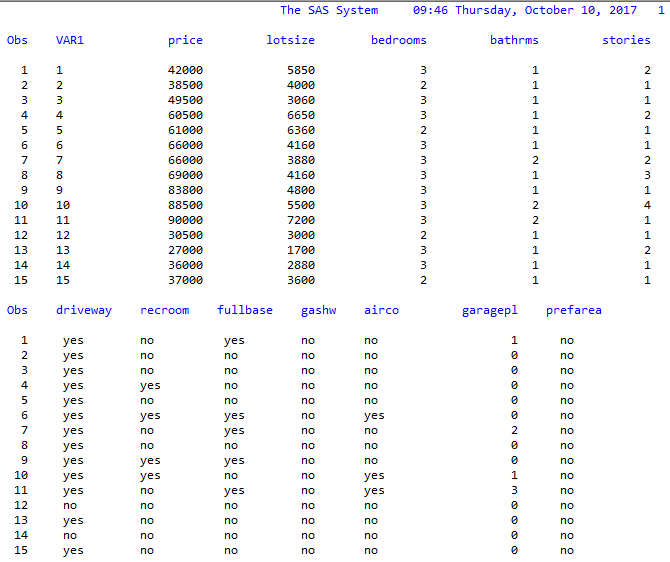
  1. Data View

sas data view.png

The first 15 observations are displayed above.

Chapter 2 A Simple Regression Model

  
  Predicting house price using its lot size. x=lot size, y=price.
SAS output
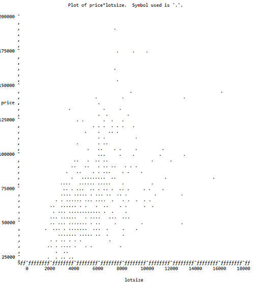
  1. Scatterplots

sas scatterplots.png

Scatterplot of price vs. lot size.

  1. Analysis of Scatterplot
  2. The Linear Regression Model
    State your regression model and briefly explain

The regression model is:
(a) the meaning of your YX term in the model;
(b) how the terms on the right-side are related to E(YX);
(c) how the terms on the right-side are related to V(YX).

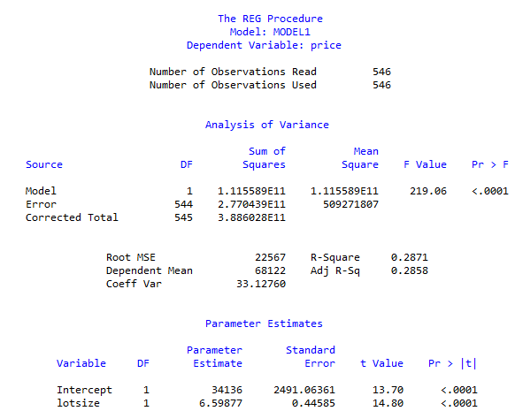
  1. SAS Output for the Fitted Model

the proc reg SAS model.png
Run Proc Reg in SAS to fit your model. Show the table output, cleaned-up, and the SAS regression plot with the confidence and prediction bands. Otherwise, only show what you are going to use.

  1. Analysis of Output
    (a) The t-tests
    (i) What is being tested?
    (ii) What are the results of the test?
    (iii) Use the Story of Many Possible Sample to explain how the test is done.

(b) The -equation

    (i) State the equation for your fitted model;
 (ii) Explain howis related to E(YX) using the story of many possible samples.

(c) In the regression plot, explain what is being shown by the 95% confidence band and the 95% prediction band. Include a vertical x-cut to provide a focus for your explanation.
A)
Download the excel dataset name online_buying. The dataset consists of purchases made by consumers across two channels from a company/firm: online and the physical store (multi-channelpurchases). More specifically, the dataset has following columns:

1) Customer: The Id of the customer.
2) Online_buy: This takes the value of 1 if the consumer buys online and 0 if he/she buys in
the physical store.
3) distance: The distance in miles from the customers home/residence to the physical store.
4) experience: The number of months that the customer has been shopping with the firm.
Thus, this can be interpreted as the experience the customer has with the firm.

5) c_rank: This is the convenience rank. Customers were asked about how convenient it
would be for them to shop online versus the physical store on a scale from 1(least
convenient) to 4 (most convenient).

  1. Formulate and estimate a (logistic) model to understand how the factors can affect the likelihood of customers shopping online. Comment on the model parameter estimates. You can calculate the odd ratios etc. What are the managerial implications of your findings?
  2. For each customer calculate the probability of him/her shopping online. You should do this based on the model estimates and the data and using the formula for p. You can do this either in excel or in SAS.

B)
Download the excel dataset brand_choice**. You have disaggregate data of choice of brands (denoted by 1, 2 and 3) in the beverage category by 50 consumers. Let’s say brands 1, 2 and 3 are Fuze, Honestea and Suja respectively. The data set consists of the following:

1) Customer_id: This denotes/indexes the customer who is making the purchase.
2) Price: This indicates the price per 12 oz. of the brand.
3) Brand: If the particular brand is chosen by the customer, then this takes the value of 1; if the brand is not chosen then this takes the value of 0.
4) Product: This number tells you which brand it is: brands 1, 2 and 3 are Fuze, Honestea
and Suja respectively.

The objective is to model the consumer’s choice of beverage brands using
brands’ pricing information. Estimate the model and interpret the results of the model.
Note: You should use proc mdc to do this.
You can modify the code given below and use it. You should first generate the intercept terms in the data for each of the products.

You can do this as follows.
In cases when product=1 then you can have int1=1 and when product=2 and product=3 then int1=0
· When product=2 then you can have int2=1 and when product=1 and product=3 then
int2=0
· When product=3 then you can have int3=1 and when product=1 and product=2 then
int3=0
So int1=1 for product 1 only and 0 otherwise; int2=1 for product 2 only and 0 otherwise; int3=1 for product 3 only and 0 otherwise. You can do the above in excel or SAS.

           proc sort data=brand_choice;
           by customer_id;
           run;
           proc mdc data=brand_choice;
           model brand = in1 in2 price /
           type=clogit
           nchoice=3;
           id customer_id;
           run;

C)

Please read the article attached (“Retailers’ Emails Are Misfires for Many Holiday Shoppers”)
and answer the following questions.

1) In your own words, what does it mean to 'personalize' digital messaging? What tools,
technologies and methods are necessary to personalize digital messaging?

2) The article says “the ugly truth is that most retailers haven’t done the unsexy work of
understanding how to use the data”. How can retailers use the data available to them to
better design personalized emails? What should they do? How can customers be targeted with the right product?

https://www.wsj.com/articles/retailers-emails-are-misfires-for-many-holiday-shoppers-1511778600

Scenario: Melbourne Property Prices

An important issue to many young Australians is housing affordability with recent
booms in property prices in Australia’s largest cities making it more difficult for
first-time homebuyers to enter the market. Sellers and buyers alike are interested in
what drives property prices, and buyers are generally interested in knowing where
bargains can be found.

We will consider data on more than 23,000 properties listed on
domain.com.au in the Melbourne metropolitan area between January 2016 and September 2017.

These data include key geographic information (e.g., suburb, address, distance from Melbourne CBD), property information (e.g., property type, number of rooms, land
and building area), and selling information (e.g., agent, sale method, price).

For this project, there are three primary questions to be investigated:

(a) Does property price increase the closer you get to the Melbourne CBD, and does the relationship between distance from the Melbourne CBD and property price change depending on the property type?

(b)What factors are most relevant in helping to predict property prices, and which
general region (REGION NAME) appears to be the best bargain for houses (i.e.
excluding other property types) based on what you would predict house prices
to be for that region?

(c)Are there certain (non-geographic) attributes of properties that characterize a
general region (REGION NAME)? In other words, is (non-geographic) information
on the property sufficient to allow a buyer to understand where a property is
likely to be located?

Expectation:
Methods and Analysis:
Provides a description of the data and the statistical analyses that will be performed. If a linear regression, principal component analysis, or linear discriminant analysis is to be carried out, this section should provide an explanation of and motivation for the variables that are included in the model. This section should also include descriptive statistics (statistics, tables, graphs) that are useful in describing the data and providing a glimpse of what you might expect from your statistical analyses. A good deal of thought should go into your descriptive statistics, as these must clearly show some relevance to your questions of interest, and you must explain what you can derive from these.

Results:
Provides a thorough description of the results of the analyses you described in the previous section. Include tables with relevant output. If analyses are carried out that involve the estimation of parameters, this should include an interpretation of the parameters for the variables of interest. Any issues with significant violations of the requirements/assumptions needed to perform the analyses carried out must be addressed.

R code and summary output should not be pasted into the document, but instead relevant results should be presented in nicely formatted tables.